이번에는 ViT 논문 리뷰에 이어서 pytorch로 구현한 내용에 대해 정리해보겠습니다.
리뷰는 아래에서 확인하실 수 있습니다.
https://vstylestdy.tistory.com/51
[논문 리뷰] ViT, An Image is Worth 16x16 Words
Vision transformer 논문에 대한 간단한 리뷰를 정리해보겠습니다. Paper : https://arxiv.org/abs/2010.11929 An Image is Worth 16x16 Words: Transformers for Image Recognition at Scale While the Transform..
vstylestdy.tistory.com
이번에 구현한 내용은 논문과 동일하게 vision transformer를 구현하고 학습시킨 것이 아니라,
CIFAR10 dataset을 이용하여 간단하게 처리 과정만을 구현한 코드입니다.
성능에 대한 실험 등은 포함되지 않고, ViT의 처리 과정을 구현하는 것에 의의를 두고 제대로 학습이 이뤄지는지에 대해서만 검사할 것입니다.
전체 코드는 아래 링크에서 확인하실 수 있고, Embedding, Transformer Encoder, MLP 최종적을 ViT module의 구현에 대해 집중적으로 살펴보겠습니다.
https://github.com/LimYooyeol/AI-Paper-Code/tree/main/ViT
- Embedding
from einops import rearrange

class Embedding(nn.Module) :
  def __init__(self, input_size = 32, input_channel = 3, hidden_size = 8*8*3, patch_size = 4) :
    super().__init__()

    self.patch_size = patch_size
    self.hidden_size = hidden_size

    self.projection = nn.Linear((patch_size**2)*input_channel, hidden_size, bias = False)

    self.cls_token = nn.Parameter(torch.zeros(hidden_size), requires_grad= True)

    num_patches = int((input_size / patch_size) ** 2 + 1)

    self.positional = nn.Parameter(torch.zeros((num_patches, hidden_size), requires_grad= True))


  def forward(self, x) :
    x = rearrange(x, 'b c (h p1) (w p2) -> b (h w) (c p1 p2)', p1 = self.patch_size, p2 = self.patch_size)
    x = self.projection(x)

    batch_size = x.shape[0]

    x = torch.concat((self.cls_token.expand(batch_size, 1, self.hidden_size), x), axis = 1)

    x = x + self.positional

    return x
먼저 CIFAR 10 dataset은 3x32x32 크기로 작기 때문에, patch size와 hidden size 또한 그에 맞춰 작게 설정했습니다.
이미지를 patch로 나누는 과정이 복잡할 것이라고 예상했는데, 'einops'를 사용하면 한 줄로 간단하게 구현할 수 있었습니다.

Input으로 주어진 images의 shape가 'batch size x channel x H x W'라고 할 때 H와 W를 각각 h, w개의 patch들로 이뤄졌다고 보고, 각각의 batch 별로 h*w 개의 c*p1*p2 크기의 vector로 만들라는 내용의 코드입니다.
Einops 자체가 직관적이라 arange로 표현된 예시와 함께 살펴보시면 이해될 것이고,
자세한 einops의 동작에 대해서는 공식문서나 튜토리얼이 있으니 찾아보면 좋을 것 같습니다.
원하던대로 image의 각 영역(patches)을 vector로 만든 것을 확인할 수 있습니다.
Cls token이나 positional embedding은 nn.Parameter를 통해 구현했고,
cls token의 경우 expand와 concat을 통해, positional embedding의 경우 broadcasting을 통해 더해줍니다.
- Transformer Encoder
● MSA (un-parallelized)
class SelfAttention(nn.Module) :
  def __init__(self, input_dim, D_h) :
    super().__init__()

    self.D_h = D_h

    self.q = nn.Linear(input_dim, D_h, bias = False)
    self.k = nn.Linear(input_dim, D_h, bias = False)
    self.v = nn.Linear(input_dim, D_h, bias = False)

    self.softmax = nn.Softmax(dim = 1)

  def forward(self, x):
    q = self.q(x)
    k = self.k(x)
    k_tranpose = torch.transpose(k, 1, 2)
    v = self.v(x)

    A = self.softmax(torch.matmul(q, k_tranpose) / (self.D_h ** (1/2)))

    return torch.matmul(A, v)

class MSA(nn.Module) :
  def __init__(self, hidden_dim = 192, num_heads = 6) :
    super().__init__()

    self.num_heads = num_heads

    heads = []
    for i in range(0, num_heads) :
      heads.append(SelfAttention(input_dim = hidden_dim, D_h = int(hidden_dim / num_heads)))

    self.heads = nn.ModuleList(heads)

  def forward(self, x):
    score = []

    for i in range(0, self.num_heads) :
      score.append(self.heads[i](x))

    return torch.concat(score, axis = 2)
먼저 Multi-head attention layer를 naive하게 구현한 코드입니다.
Self-attention head를 먼저 구현하고, MSA에서는 여러 개의 heads를 ModuleList로 저장하여, 하나씩 계산한 결과를 이어 붙입니다.
따라서 head 별 연산이 sequential하게 이뤄져서 비효율적입니다.
● MSA(Parallelized)
병렬화 된 버전의 구현은 https://github.com/FrancescoSaverioZuppichini/ViT/blob/main/transfomer.md 의 코드를 이용했습니다.
여기에서도 einop의 rearrange와 torch.einsum을 이용하는데, 먼저 코드는 다음과 같습니다.
# https://github.com/FrancescoSaverioZuppichini/ViT/blob/main/transfomer.md
class MSA(nn.Module) :
def __init__(self, hidden_dim = 8*8*3, num_heads = 6) :
super().__init__()
self.num_heads = num_heads
self.D_h = (hidden_dim / num_heads) ** (1/2)
self.queries = nn.Linear(hidden_dim, hidden_dim)
self.keys = nn.Linear(hidden_dim, hidden_dim)
self.values = nn.Linear(hidden_dim, hidden_dim)
self.softmax = nn.Softmax(dim = 1)
def forward(self, x) :
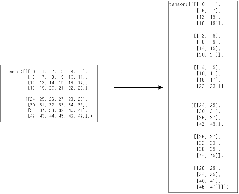
q = rearrange(self.queries(x), 'b n (h d) -> b h n d', h = self.num_heads)
k = rearrange(self.queries(x), 'b n (h d) -> b h n d', h = self.num_heads)
v = rearrange(self.queries(x), 'b n (h d) -> b h n d', h = self.num_heads)
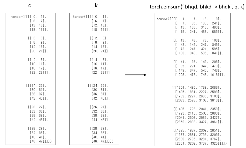
A = torch.einsum('bhqd, bhkd -> bhqk', q, k)
A = self.softmax(A / self.D_h)
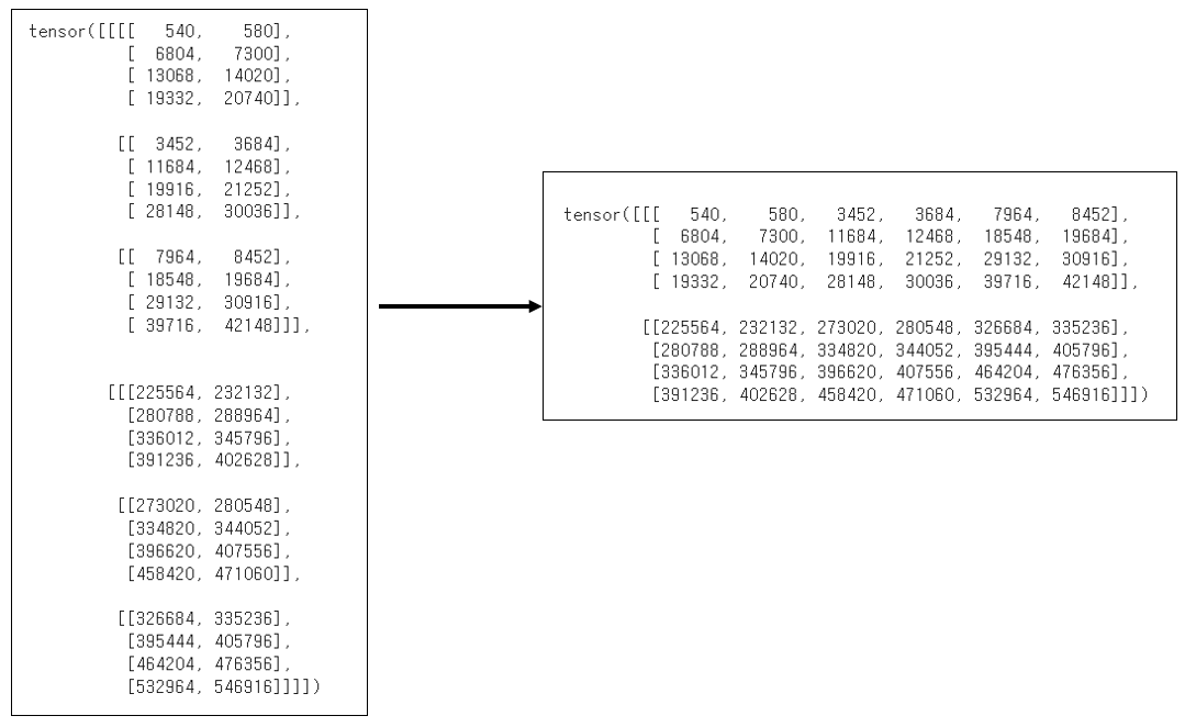
Ax = torch.einsum('bhan, bhnd -> bhad' ,A, v) # b : batch size, h : num_heads, n : num_patches, a : num_patches, d : D_h
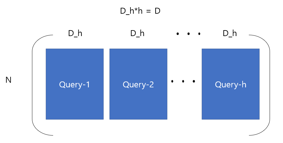
return rearrange(Ax, 'b h n d -> b n (h d)')먼저 query, key, value weights를 nn.Linear layer로 선언하는데, 이번엔 모든 heads의 weights를 하나의 layer로 처리하기 때문에 output의 크기로 D(hidden dim)가 유지됩니다.
즉, 각 헤드별로 NxDh, (N x D) x (D x Dh)의 결과를 생성하는 것을 한번에 N x D로 처리합니다.
따라서 forward weight를 거친 결과는 다음과 같게 됩니다.(query 기준, h : # of heads)
● MLP
class MLP(nn.Module):
  def __init__(self, input_dim = 8*8*3, hidden_dim = 8*8*3*4, output_dim = 8*8*3):
    super().__init__()

    self.feedforward = nn.Sequential(
        nn.Linear(input_dim, hidden_dim),
        nn.GELU(),
        nn.Linear(hidden_dim, output_dim),
        nn.GELU()
    )

  def forward(self, x) :
    return self.feedforward(x)
MLP는 2 layer net이라고 보면 됩니다. Input과 output의 크기는 같고, 중간에 숨겨진 hidden dim은 임의로 input의 4배 정도로 설정해주었습니다.
(여기에서만 hidden dim은 hidden layer의 차원을 의미하고 그 외에는 D, encoder 전체에서 흐르는 vector의 dimension을 의미합니다.)
● TransformerEncoderBlock, TransformerEncoder
class TransformerEncoderBlock(nn.Module) :
  def __init__(self, hidden_dim = 8*8*3, num_heads = 6, mlp_size = 8*8*3*4):
    super().__init__()

    self.LN = nn.LayerNorm(normalized_shape= hidden_dim)
    self.MSA = MSA(hidden_dim = hidden_dim, num_heads = num_heads)
    self.MLP = MLP(input_dim = hidden_dim, hidden_dim = mlp_size, output_dim = hidden_dim)

  def forward(self, x) :
    x_prev = x
    x = self.LN(x)
    x = self.MSA(x)

    x = x + x_prev
    x_prev = x

    x = self.LN(x)
    x = self.MLP(x)

    return x + x_prev
LN -> MSA -> LN -> MLP가 이어지는 block 입니다. 중간중간 residual connection도 추가해줍니다.
class TransformerEncoder(nn.Module):
  def __init__(self, hidden_dim = 8*8*3, num_layers = 8) :
    super().__init__()

    self.num_layers = num_layers
    self.hidden_dim = hidden_dim

    layers = []

    for i in range(0, num_layers) :
      layers.append(TransformerEncoderBlock())

    self.blocks = nn.ModuleList(layers)

    self.LN = nn.LayerNorm(normalized_shape= hidden_dim)

  def forward(self, x):
    for i in range(0, self.num_layers) :
      x = self.blocks[i](x)

    return self.LN(x[:, 0, :])
Encoder는 앞서 구현한 transformer encoder block이 L개 연속되도록 구현해줍니다.
여기에서도 ModuleList를 이용하여 구현해주었습니다.
Encoder의 output은 classification token에 대한 마지막 block의 출력입니다.
- MLP Head
class MLPHead(nn.Module) :
  def __init__(self, input_dim = 8*8*3, hidden_dim = 8*8*3*4, num_classes = 10) :
    super().__init__()

    self.feedforward = nn.Sequential(
        nn.Linear(input_dim, hidden_dim),
        nn.ReLU(),
        nn.Linear(hidden_dim, num_classes)
    )

  def forward(self, x) :
    return self.feedforward(x)
Classification을 위한 MLP head 에서는 encoder의 output을 input으로 받아 classifciation을 수행하면 됩니다.
일반적인 2 layer net입니다.
- ViT
최종 ViT는 다음과 같이 Embedding - Transformer Encoder - MLP Head가 이어지는 구조입니다.
class ViT(nn.Module) :
  def __init__(self, input_size = 32, patch_size = 4, hidden_size = 8*8*3, num_layers = 8) :
    super().__init__()

    self.vit = nn.Sequential(
        Embedding(input_size = input_size, input_channel = 3, hidden_size = hidden_size, patch_size = patch_size),
        TransformerEncoder(hidden_dim = hidden_size, num_layers = num_layers),
        MLPHead(input_dim = hidden_size, hidden_dim = hidden_size*4, num_classes= 10)
    )

  def forward(self, x):
    return self.vit(x)
- Training
Optimizer는 Adam을 사용했고, lr = 1e-3, (B1, B2) = (0.9, 0.99)를 사용했습니다.
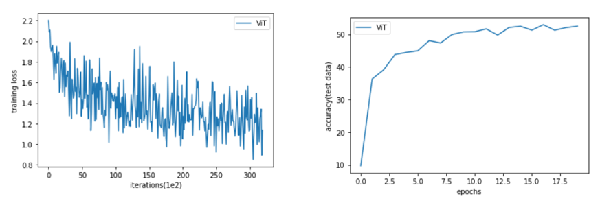
학습이 잘 이뤄지는 것을 확인할 수 있습니다.
아직 수렴하지 않았지만, 처음에 언급했듯이 연산을 구현해보는 것이 목적이었기 때문에 training은 20 epochs에서 더 진행하지 않았습니다.
'Computer Vision > 공부' 카테고리의 다른 글
| [논문 리뷰] ViT, An Image is Worth 16x16 Words (0) | 2022.02.05 |
|---|---|
| [논문 리뷰/구현] ResNet (0) | 2022.01.28 |