※ 본 내용은 stanford에서 제공하는 cs231n 강의, 강의자료를 바탕으로 작성하였습니다.
Q3에서는 Softmax loss의 구현과 SGD에 대해 다루고 있다.
Q2와 비슷한 구조로, naive하게 loss와 미분을 계산하는 것에서 fully vectorized한 코드까지 작성하는 것을 다룬다.
(SGD를 이용한 train의 경우 Q2와 동일하므로 생략)
<Softmax>
- Setup

마찬가지로 CIFAR10 dataset을 load하여 사용하고, shape는 위와 같다.
- Naive하게 loss와 미분(dW) 계산하기
def softmax_loss_naive(W, X, y, reg):
    """
    Softmax loss function, naive implementation (with loops)

    Inputs have dimension D, there are C classes, and we operate on minibatches
    of N examples.

    Inputs:
    - W: A numpy array of shape (D, C) containing weights.
    - X: A numpy array of shape (N, D) containing a minibatch of data.
    - y: A numpy array of shape (N,) containing training labels; y[i] = c means
      that X[i] has label c, where 0 <= c < C.
    - reg: (float) regularization strength

    Returns a tuple of:
    - loss as single float
    - gradient with respect to weights W; an array of same shape as W
    """
    # Initialize the loss and gradient to zero.
    loss = 0.0
    dW = np.zeros_like(W)

    #############################################################################
    # TODO: Compute the softmax loss and its gradient using explicit loops.     #
    # Store the loss in loss and the gradient in dW. If you are not careful     #
    # here, it is easy to run into numeric instability. Don't forget the        #
    # regularization!                                                           #
    #############################################################################
    # *****START OF YOUR CODE (DO NOT DELETE/MODIFY THIS LINE)*****

    # -- loss, dW --
    num_train = X.shape[0]

    for i in range(num_train) :
      score = np.dot(X[i], W)
      score = np.exp(score)
      score = score / np.sum(score)

      X_temp = np.repeat(X[i].reshape(-1, 1), 10, axis = 1)

      dW += X_temp*score / num_train # 3072x10
      dW[:, y[i]] += -X[i] / num_train

      loss += -np.log(score[y[i]])

    dW += 2*reg*W

    loss /= num_train
    loss += reg*np.sum(W*W)

    # *****END OF YOUR CODE (DO NOT DELETE/MODIFY THIS LINE)*****

    return loss, dW
loss와 미분을 naive하게 구현하는 코드는 위와 같다.
● Softmax Loss
for문을 사용하여 loss는 직관적으로 구현되어 있다. 계산 방법을 순서대로 코드화한 것 뿐이라 크게 어렵지 않다.
● 미분(dW)
처음엔 Softmax에서 Weight(W)에 대한 미분을 어떻게 계산해야 할지 감이 안왔지만,
SVM에서 했던 것과 유사하게 loss에 더해지는 값을 풀어쓴 후 미분할 수 있었다.
각 데이터마다 loss에 더해지는 값은 다음과 같다.
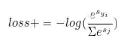
(s_x는 x-th class에 대한 prediction score, y_i는 정답 label을 의미한다.)
이를 좀 더 풀어보면,


위와 같이 정리할 수 있다.
따라서 각 데이터마다 $ dW^{(i)}$에 대한 미분은 위식을 $ W^{i}$에 대해 미분한 결과와 같다.
score가 데이터와 Weight의 내적인 점을 고려하여 미분을 진행하면 최종적으로 다음과 같은 식이나온다.
$ dW^{(i)} += x^{(n)}*probability(i) $ (i가 정답 label이 아닌 경우)
$ dW^{(i)} += -x^{(n)} + x^{(n)}*probability(i) $ (i가 정답 label인 경우)
다항식과 log로 이뤄진 복잡하지 않은 식이라, 자세한 미분과정은 생략하였다.
추가적으로 data의 수로 나눠주고, regularization term에 대한 미분을 더해주면 미분 계산이 완료된다.
코드는 단순히 위 내용을 구현한 내용이라 자세히 설명하진 않겠다.
- Inline Question 1

위 결과가 -log(0.1)과 비슷한지 검사하는 내용이 있었는데, 왜 해당 값과 비교하는지 설명하라는 질문이 있었다.
- Fully vectorize하여 loss와 미분 계산하기
def softmax_loss_vectorized(W, X, y, reg):
    """
    Softmax loss function, vectorized version.

    Inputs and outputs are the same as softmax_loss_naive.
    """
    # Initialize the loss and gradient to zero.
    loss = 0.0
    dW = np.zeros_like(W)

    #############################################################################
    # TODO: Compute the softmax loss and its gradient using no explicit loops.  #
    # Store the loss in loss and the gradient in dW. If you are not careful     #
    # here, it is easy to run into numeric instability. Don't forget the        #
    # regularization!                                                           #
    #############################################################################
    # *****START OF YOUR CODE (DO NOT DELETE/MODIFY THIS LINE)*****

    #loss
    score = np.dot(X, W) # 500 x 10
    score = np.exp(score)
    score = score / np.sum(score, axis = 1).reshape(-1, 1)
    loss = np.sum(-np.log(score[np.arange(X.shape[0]), y])) / X.shape[0] + reg*np.sum(W*W)


    #dW
    score[np.arange(X.shape[0]), y] -= 1 #not valid from here
    dW += np.dot(np.transpose(X), score) / X.shape[0]  # 3072x10
    dW += 2*reg*W

    # *****END OF YOUR CODE (DO NOT DELETE/MODIFY THIS LINE)*****

    return loss, dW
for문을 사용하지 않고, vectorization을 통해 구현한 코드는 위와 같다.
● Loss
loss의 경우 사실 처음부터 vectorized version으로 작성하는 것이 편했다.
score의 shape가 어떻게 결정되는지만 이해했다면 쉽게 이해할 수 있을 것이다.
앞서 각 데이터별로 for문을 거치며 계산한 과정을 행렬에 저장된 결과를 보고 계산한 것 뿐이다.
● 미분
앞서

위와 같은 수식을 확인할 수 있었다.
i번째 W에 대한 미분을 구하려면 n번째 데이터와 해당 데이터의 i-th class에 대한 score의 곱을 모든 데이터에 대해 더해주면 된다. i가 정답인 경우는 probability에 -1을 더해줘서 곱하면 된다.
앞서 Q2에서 모든 데이터에 각각 어떤 값을 곱하고, 그 합을 구하는 것을 for문을 사용하지 않고 구현하는 코드가 있었고, 해당 코드와 동일한 원리로 행렬곱을 이용해 계산할 수 있었다.
X의 전치행렬과 확률이 계산된 행렬을 곱해주면 되었다. (정답 label인 경우 확률에 -1을 해줘야한다.)

위 그림은 $ dW^{(0)}$를 계산하는 예시로, 그림을 통해 확인하면 보다 쉽게 이해할 수 있을 것이다.
마지막으로 regularization term에 대한 미분을 더해주면 fully vectorized된 미분 계산 코드를 완성할 수 있다.
'Computer Vision > cs231n' 카테고리의 다른 글
| [Assignment1 - Q4] 2-layer NN (0) | 2022.01.01 |
|---|---|
| [Lec 4] Backpropagation and Neural Network (0) | 2021.12.30 |
| [Assignment1 - Q2] SVM (0) | 2021.12.30 |
| [Lec 3] Loss Functions and Optimization (0) | 2021.12.30 |
| [Assignment 1 - Q1] KNN (0) | 2021.12.29 |